DM-EFD prototype implementation based on Kafka and InfluxDB.
Note
This technote is not yet published.
1 Introduction
In DMTN-082 we sketched out a proposed solution to the problem of exposing data like telescope telemetry to the Science Platform users with minimal latency. This is a usecase that arose from the desire to make Science Platform capabilities to the Commissioning team, which requires prompt access to observatory parameters during characterisation of the facility. We therefore sketched out an architecture based on Kafka to siphon the data from the SAL writers (who populate the Engineering Facilities Database) to a time-series database. During review of this proposal, the DM Manager asked for a demonstration that this architecture would be capable of scaling to the required data throughput.
We developed a prototype to demonstrate the elements of this architecture and to be able to benchmark its performance. The results of this prototype sprint are described in this report. The purpose of this report is to inform the decision on whether to proceed with this architecture.
2 The adopted technologies
2.1 The Confluent Kafka platform
We adopted the open source Confluent Platform Helm charts specifically as the canonical Kubernetes-based Kafka distribution for this investigation. The platform consists of the following components:
- Kafka broker and Zookeeper cluster
- Confluent Schema Registry service
- Kafka Connect server
- KSQL server
- Confluent REST Proxy
The Kafka brokers are the core of the Kafka service. Kafka brokers receive messages from producers, store that data on disk, and provide messages to consumers. Kafka brokers are effectively databases. The Zookeeper cluster manages the Kafka cluster.
The Schema Registry is a unique product developed by Confluent that provides an HTTP API for a database of Avro schemas that define the format of messages in Kafka topics (the schemas themselves are persisted as Kafka topics). In short, Avro and the Schema Registry enable us to efficiently encode messages with full knowledge of the format of those messages. Schemas are versioned so that the content of topics can evolve over time, without breaking the ability to read older topics. Avro and the Schema Registry are discussed further in 4 SAL schema management with Avro and the Schema Registry.
Kafka Connect is another product developed by Confluent that allows us to deploy ready-made services that move Kafka messages to and from other services. Kafka Connect makes use of Avro and the Schema Registry to make data formatting issues completely transparent. Confluent maintains a central listing of connectors at https://www.confluent.io/hub/. For this investigation, we use the Landoop InfluxDB connector, which moves Kafka messages to InfluxDB in real time (see the next section for an introduction to InfluxDB).
KSQL is another product developed by Confluent and included in the platform deployment KSQL provides a SQL-like query engine on top of Kafka topics. We have not yet made use of it in this investigation as InfluxDB provides our primary query platform, though it is an interesting capability.
The REST Proxy, as the name suggests, provides an HTTP API for producing or consuming Kafka messages. Since the Kafka design normally requires clients to have network visibility to all brokers in a cluster, it’s difficult to expose brokers to the internet. The REST Proxy provides one solution to it, though we have not used it in this investigation.
All of these services are deployable from a set of Helm charts that are maintained by Confluent. We have also been able to wrap the Helm deployment with Terraform, to make a customized infrastructure-as-code solution for our specific Kafka deployments. As a result, we have found it quite easy to stand up and operate Kafka and related services in Kubernetes. See 3.3 Terraform and Helm for further discussion.
2.2 The InfluxData stack
2.2.1 Why a time-series database?
Telemetry data and events are, by nature, time-series data.
A time-series database (TSDB), in contrast to a general purpose relational database like MySQL or Oracle, is already optimized to efficiently store and query time-series data. A TSDB like InfluxDB already implements features like data retention policies and downsampling which are fundamental to the time-series data management.
A TSDB stores data in shards indexed by the timestamp which makes queries constrained by a time interval extremely efficient.
2.2.2 Why InfluxData?
The InfluxData stack provides a complete solution for storing, visualizing and processing time series data:
- InfluxDB is an open-source time series database written in Go, it has an SQL-like query language (InfluxQL) and provides an HTTP API as well as API client libraries.
- Chronograf is an open-source web application for time series visualization written in Go and React.js
- Kapacitor is an open-source framework written in Go for processing, monitoring, and alerting on time series data.
3 Deploying Confluent Kafka and InfluxData
3.1 The GKE cluster specs
- Machine type: n1-standard-2 (2 vCPUs, 7.5 GB memory)
- Size: 3 nodes
- Total cores: 6 vCPUs
- Total memory: 22.50 GB
The above specs are sufficient for running JVM, but not recommended for production. See Running Kafka in Production and InfluxDB hardware guidelines for single node for more information.
3.2 InfluxDB hardware guidelines
Based on the expected throughput from SAL (see 6 The mock SAL experiment), the InfluxDB performance requirements fall into the moderate load category. Thus a single InfluxDB node for each instance of the DM-EFD is enough.
Considering that monitoring of the DM-EFD data during operations will require more than 25 moderate queries per second, we probably should be more conservative and follow the high load hardware sizing recommendations:
- CPU: 8+ cores
- RAM: 32+ GB
- IOPS: 1000+
It is also recommended that InfluxDB should be run on locally attached solid state drives (SSDs) to increase I/O performance. Note that more tests should be done beyond this prototype implementation to estimate the hardware sizing if Kapacitor is used to aggregate the time-series data.
3.3 Terraform and Helm
We have used a combination of Terraform and Helm to automate the creation of the cluster on GKE and to install the Confluent Kafka and InfluxDB applications (see terraform-efd-kafka). It also includes the installation of a Grafana dashboard for monitoring system metrics.
The creation of the InfluxDB database and retention policies, the creation of the InfluxDB sink connector, the initializion the SAL topics in the Kafka Schema Registry, and the deployment of the SAL transformers is also automated by installing the kafka-efd-apps Helm chart.
In summary, the deployment of the DM-EFD is done after setting a small number of configuration parameters and executing a single Terraform command that creates 32 resources in a few minutes.
4 SAL schema management with Avro and the Schema Registry
This section describes how message schemas are managed.
4.1 SAL schema background
To review, SAL organizes messages into topics. Topics belong to subsystems and can be categorized as telemetry, events, or commands. As of January 25, 2019, there are 1228 topics across 66 subsystems. Messages within a topic share a schema and these schemas are developed and published as XML files in the ts_xml repository on GitHub.
Note
Our understanding is that these XML files are part of the SAL build process. The SAL codebase is templated so that individual writers for different subsystems are dynamically coded and compiled in response to the ts_xml schemas.
SAL topic schemas can evolve (certainly, they do evolve within the ts_xml Git repository). However, we do not know how schemas can evolve, if at all, within an operational SAL system.
We are also thus far unaware of how to identify the version of a schema given an operation SAL system, or from a SAL message itself.
These schemas define the content of a SAL message, though they do not prescribe an encoding for that content. Our understanding is that SAL receives messages from devices on the DDS bus in a specific binary format conforming to the ts_xml schemas, and then SAL writers transform those messages into other formats for different users. For example, the SAL’s EFD writer transforms DDL messages into SQL insert commands for the EFD itself.
4.2 The role of Avro
In the present investigation, Kafka becomes another user of the SAL, equivalent and analogous to the SQL-based EFD itself. Kafka does not prescribe a specific format for its messages — any binary content can be transmitted as a Kafka message. That said, it’s quite common to use Avro as the serialization format for Kafka messages. Avro is a data serializations system that uses schemas written in JSON. We note that the DM Alert Stream also uses Avro to serialize data in messages (see DMTN-093: Design of the LSST Alert Distribution System). Avro has a flexible typing system that accommodates simple types like strings, integers, floats and booleans, container types like arrays, mappings, records, and complex types like semantic timestamps. Avro schemas also support arbitrary metadata, which is convenient for transcribing the ts_xml schemas (see 4.4 Systematic conversion of SAL Avro schemas).
One of the most compelling features of Avro is that schemas can be designed to allow forwards and backwards compatibility for message producers and consumers if a schema changes:
- Backwards compatibility
Backwards compatibility means that a schema written with an older version of a schema can be read by a consumer that uses a newer version of a schema. To revise a schema in a backwards-compatible way, you can delete fields or add optional fields (that have defaults).
A consumer reading an older message wouldn’t see any values from the deleted field, and would see the default value for any new fields.
- Forwards compatibility
Forwards compatibility means that a producer can create a message with a newer version of a schema, and that message could still be read by a consumer that expects data serialized with an older version of a schema. To revise a schema in a forwards-compatible way, you can add fields or delete optional fields.
The consumer wouldn’t see the new fields, and would see default values for the deleted optional fields.
- Full compatibility
A combination of backwards and forwards compatibility, fully-compatible schema changes mean that either the producer (SAL) or the consumer (InfluxDB, for example) can be upgraded first.
To revise schemas at this level of compatibility, only optional fields can ever be added or deleted.
- Transitive compatibility
- Compatibility can also be required to be transitive. This means that any type of compatibility is true not only between two versions of a schema, but for all versions of a schema.
Additionally, Avro allows fields to be renamed by designating aliases for the names of fields.
Overall, implementing a regulated schema evolution system implemented through Avro means that SAL and consumers of SAL’s Kafka topics can be upgraded independently. For more discussion, see the Confluent documentation on Schema Evolution and Compatibility. Later in this section we also discuss compatibility requirements for the DM-EFD specifically.
4.3 The role of the Schema Registry
The Confluent Schema Registry makes Avro schemas and messages serialized with those schemas much easier to use.
By providing an easily accessible HTTP API for retrieving schemas, individual schemas don’t need to include a copy of the schema in order to be fully self-describing. Instead, messages are encoded in the Confluent Wire Format where the first several bytes of the message include the unique ID of the message’s schema in the registry. Thus a consumer can always retrieve a message’s schema by querying the Schema Registry.
Second, the Schema Registry organizes schemas semantically to allow versioning. In a Schema Registry a subject is a named entity that tracks a versioned set of schemas. Subjects can be configured with compatibility requirements (see the previous section). By default, new versions of schemas in a subject are required to have backwards compatibility. Forwards, full, and transitive variants, of compatibility requirements can also be configured. Or even no compatibility.
Note
The same schema (as identified by its unique ID) can belong to multiple subjects.
Our convention is to name these subjects after the fully-qualified names of the schemas in them.
For example, the namespace of all schemas for SAL topics is lsst.sal.
For a topic named MTM1M3TS_thermalData the fully-qualified schema name, and subject name, is lsst.sal.MTM1M3TS_thermalData.
4.4 Systematic conversion of SAL Avro schemas
We have built the capability to automatically transform the original SAL schemas in ts_xml to Avro schemas hosted in the Schema Registry. The capability is included in kafka-efd-demo, our demonstration Python package for the present investigation. The schema conversion command uses the GitHub HTTP APIs to download schemas corresponding to an arbitrary branch or commit of the ts_xml repository.
We believe that Avro can reliably represent all field types described in the ts_xml schemas (though we have not yet seen actual data from all SAL topics, yet). The next three sections describe how ts_xml schemas are automatically converted, at both the level of a message, and for individual fields within that message.
4.4.1 Conversion of topic schemas
In ts_xml, topic schemas are defined in SALCommand, SALEvent, or SALTelemetry tags.
In practice, all three types of topics are structured similarly, and the same conversion algorithm applies to each.
The following table shows how tags with SALCommand, SALEvent, or SALTelemetry tags are mapped into Avro schemas.
| SAL tag | Avro schema key | Note |
|---|---|---|
| EFDB_topic | name | Core Avro key |
| namespace | Default: lsst.sal |
|
| Explanation | doc | Core Avro key |
| item, … | fields | Core Avro key, see 4.4.2 Conversion of field schemas |
| sal_topic_type | Custom Avro metadata, one of SALCommand, SALEvent, or SALTelemetry |
|
| Subsystem | sal_subsystem | Custom Avro metadata |
| Version | sal_version | Custom Avro metadata |
| Author | sal_author | Custom Avro metadata |
| Alias | sal_alias | Custom Avro metadata |
| Device | sal_device | Custom Avro metadata |
| Property | sal_property | Custom Avro metadata |
| Action | sal_action | Custom Avro metadata |
| Value | sal_action | Custom Avro metadata |
Note that the name and namespace, when combined, form the fully-qualified schema name.
An example is lsst.sal.MTM1M3TS_thermalData where MTM1M3TS_thermalData is a telemetry topic in the MTM1M3TS subsystem.
These fully-qualified schemas names are, by our convention, the name of the corresponding subject in the Confluent Schema Registry.
Avro keys that are prefixed with sal_ aren’t part of the core Avro schema specification, but do allow us to include metadata content from the ts_xml schemas in Avro schemas.
Remember that these keys are metadata associated with the schema, and aren’t included in the messages.
Message content is defined by the fields, described next.
4.4.2 Conversion of field schemas
Topic schemas, in addition to the metadata described above, consist principally of a list of fields. The following table describes how individual tags within a ts_xml field are converted to Avro metadata.
| SAL tag | Avro field key | Note |
|---|---|---|
| EFDB_Name | name | Core Avro key |
| Description | doc | Core Avro key |
| IDL_type | type | See section text |
| Units | sal_units | Custom Avro metadata |
| Frequency | sal_frequency | Custom Avro metadata |
| Publishers | sal_publishers | Custom Avro metadata |
| Values_per_Publisher | sal_values_per_publisher | Custom Avro metadata |
| Size_in_bytes | sal_size_in_bytes | Custom Avro metadata |
| Conversion | sal_conversion | Custom Avro metadata |
| Sensor_location | sal_sensor_location | Custom Avro metadata |
| Instances_per_night | sal_instances_per_night | Custom Avro metadata |
| Bytes_per_night | sal_bytes_per_night | Custom Avro metadata |
| Needed_by_DM | sal_needed_by_dm | Custom Avro metadata |
| Needed_by_Camera | sal_needed_by_camera | Custom Avro metadata |
| Needed_by_OCS | sal_needed_by_ocs | Custom Avro metadata |
| Needed_by_TCS | sal_needed_by_tcs | Custom Avro metadata |
| Needed_by_EPO | sal_needed_by_epo | Custom Avro metadata |
| sal_index | Custom Avro key that enumerates the order of the field in the XML schema. |
Note that not all of the “custom” Avro keys appear in all schemas.
Most work involved in converting a ts_xml schema is associated with converting type information. For elementary data types, the conversion code simply maps the DDS types for fields listed in ts_xml to Avro types (Table 3).
| Avro | DDS |
|---|---|
| null | null |
| boolean | boolean |
| string | string |
| int | int, unsigned int, short, unsigned short |
| long | long, long long, unsigned long, unsigned long long |
| bytes | bytes, byte, char, octet |
In cases where a field in a ts_xml schema has a Count tag with a value greater than 1, then that field is interpreted as an array.
Avro arrays can have items of any type described above.
The ts_xml schemas can also include fields that are enumerations, where the value is one of a finite number of symbols.
Avro natively supports these enumerations.
For example, PointingComponent_command_raDecTarget topic includes a field named targetInstance.
In XML, this field is described as:
<item>
    <EFDB_Name>targetInstance</EFDB_Name>
    <Description>Which target: is being defined (current or next)</Description>
    <IDL_Type>long</IDL_Type>
    <Enumeration>current,next,prospective</Enumeration>
    <Units/>
    <Count>1</Count>
</item>
The Avro conversion is:
{
  "doc": "Which target: is being defined (current or next)",
  "name": "targetInstance",
  "sal_index": 1,
  "type": {
    "name": "targetInstance",
    "symbols": [
      "current",
      "next",
      "prospective"
    ],
    "type": "enum"
  }
}
Not all fields in ts_xml are set up to have machine-readable enumerations.
For example, the PointingComponent_command_copyTarget topic has two fields:
<item>
    <EFDB_Name>copyFrom</EFDB_Name>
    <Description>Target definition will be copied from this target. The 'to' and 'from' targets must be different.</Description>
    <IDL_Type>long</IDL_Type>
    <Enumeration>current,next,prospective</Enumeration>
    <Units/>
    <Count>1</Count>
</item>
<item>
    <EFDB_Name>copyTo</EFDB_Name>
    <Description>Target definition will be copied to this target. The 'to' and 'from' targets must be different. Use the same enumeration constants as copyFrom.</Description>
    <IDL_Type>long</IDL_Type>
    <Units/>
    <Count>1</Count>
</item>
Of these, the Avro schema identifies the copyFrom field as an enumeration, but the copyTo field as a regular long-type field.
This practice of documenting enumerations in the free-form description of a field, rather than with an embedded Enumeration tag is fairly common in ts_xml.
The DM-EFD effort would benefit from having enumerations consistently defined in the XML schemas.
4.4.3 Additional fields in Avro schemas
In addition to the fields defined in the ts_xml schemas, the Avro schemas include additional fields to convey additional data with each message:
kafka_timestamp- This field can be used to encode timestamp when a DM application processed a Kafka message. For example, in the SAL message transformation step, this timestamp can represent when the transformation application converts a message from plain text to Avro. This field can be repurposed or eliminated in later phases of the DM-EFD project.
sal_revcode- Revision of the SAL code.
sal_created- Timestamp when SAL created the original Kafka message.
sal_ingested- Timestamp when SAL ingested the message from the DDS bus.
sal_origin- SAL origin.
sal_host- SAL host.
The last five fields are emitted by SAL with each message.
4.5 Practical approaches to integrating Avro into the SAL and DM-EFD system
Kafka and Avro aren’t initial features of the SAL. Through this investigation, the Telescope & Site team added a basic capability for SAL to produce Kafka messages by creating a Kafka writer that is analogous to existing EFD and log writers. At the moment of this writing, SAL does not encode messages in Avro. This section describes the pros and cons of two approaches to integrating Avro serialization with SAL.
4.5.1 Approach 1: online message transformation
The simplest approach, from the point of view of the SAL codebase itself, is for SAL to produce Kafka messages in a plain text format. Then a set of applications operated by DM consume, parse, and transform those messages into Avro serializations. Those transformer applications then publish the new stream of messages to a new Kafka topic (or topics) that downstream applications like the InfluxDB Kafka Connector can consume. Such a transformation can be done in real-time; as long as the transformation application can keep up with the original data rates from SAL, the transformation step introduces only a small latency to the messages. This approach has already been successfully implemented, and the results are discussed in 7 Live SAL experiment with Avro transformations.
The advantages of this approach are:
- Operation of the Schema Registry and production of Avro schemas remain under the technical control of the DM subsystem. Since DM is the sole user of Avro-serialized messages from SAL, DM is the most motivated organization to ensure that Avro serialization infrastructure is well-maintained.
- If the ts_xml schemas evolve, the DM SQuaRE team has the expertise to ensure that new versions of the corresponding Avro schemas can be compatible with earlier Avro schemas.
- The SAL application does not need extra code to interact with the Schema Registry, nor extra code to serialize messages with those schemas. In fact, the current implementation of the Kafka writer for SAL publishes messages based on plain text SQL insert commands (adapted from the EFD writer). Overall, this minimizes the Kafka-related development commitment for the SAL developers.
- The DM SQuaRE team already has experience and made investments in Python-based infrastructure for consuming and producing Kafka topics and interacting with the Schema Registry.
- If consumers of the Kafka topics need additional transformations of the messages from the SAL, these transformer apps are already in place.
The downsides of this approach are:
- The Kafka brokers must support roughly twice the message volume compared to the original SAL volume. The Kafka cluster sizing and message retention policy would need to be designed with this in mind.
- The SAL and DM-EFD teams would need to coordinate schema migration events. When SAL is deployed with a new version of ts_xml, the DM operators would register the new schemas in the Schema Registry and make any adjustments for schema compatibility requirements.
4.5.2 Approach 2: SAL produces Avro-serialized messages
The alternative approach is to build Avro schema management into SAL itself. Generally speaking SAL would need to be modified as follows:
- When SAL is compiled against the ts_xml schemas, the SAL compiler would also need to convert the XML schemas to Avro and register those schemas with the Schema Registry. Based on how SAL is currently designed, we believe that the actual Avro schemas and their corresponding IDs would be hard-coded into the Kafka writers.
- The SAL Kafka writers would need to format messages into a JSON-like data structure that the Avro serializer can operate on. Then the Kafka writer would further format the message in the Confluent Wire Format to embed the schema ID with the message before producing it.
The advantages of this approach are:
- The system is technically simpler and more integrated. If SAL is compiled against a new version of the of the ts_xml schemas, those new schemas are automatically translated and registered with the Schema Registry as part of SAL’s build process.
The downsides of this approach are:
- The SAL’s templated build system means that the DM SQuaRE team can’t effectively contribute code to SAL. Either DM SQuaRE would invest in learning how to develop SAL, or the Telescope & Site team would effectively become the sole developers and operators of code that builds Avro schemas and registers those schemas with the registry.
- The Telescope & Site team may not want to accept the added complexity in SAL.
- If DM requires that Avro schemas maintain compatibility with earlier schemas, those compatibility requirements would need to be considered before changes to ts_xml are committed. For example, a continuous integration server would test ts_xml pull requests to ensure that the XML schema changes are compatible with schemas already registered in the Schema Registry. Again, this would add some complexity to the SAL development process that primarily benefits only the DM team.
- DM either loses the ability to transform the SAL messages before ingest into InfluxDB or consumption by other applications. DM may need to deploy online stream transformation applications regardless.
4.6 What kinds of schema compatibility do we need?
As described above, Avro schemas can be versioned and those versions can be made compatible. The Schema Registry can even enforce that compatibility requirement. In typical applications, it’s straightforward to write schemas that meet compatibility requirements. The DM-EFD is atypical, though, because the Avro schemas follow the ts_xml schemas. If schema compatibility is required for DM applications, that compliance with the compatibility requirements needs to be absorbed by at least some part of the system: either the ts_xml schemas are only migrated in ways that yield compatible changes for Avro schemas, or there is manual curation of the Avro schemas to ensure compatibility.
On the other hand, it’s not immediately obvious that formal schema version compatibility is required by DM. First, since the Kafka messages are encoded in the Confluent Wire Format, each message identifies the schema that it was serialized with, and therefore the message can always be deserialized. Second, InfluxDB is intrinsically schemaless (see 5.1 The InfluxDB schema).
Further requirement and design definition work is needed to drive Avro schema management policy.
5 Connecting Kafka and InfluxDB
As of January 2019, the Confluent InfluxDB connector was still in preview and did not have the functionality we needed. Instead of the Confluent InfluxDB connector, we used the InfluxDB Sink connector developed by Landoop.
We added the Landoop InfluxDB Sink connector plugin version 1.1 to the cp-kafka-connect container and implemented scripts to facilitate its configuration.
A limitation of version 1.1, though, was the lack of support for the Avro array data type, which was solved by contributing to the plugin development.
5.1 The InfluxDB schema
One of the characteristics of InfluxDB is that it creates the database schema when it writes the data to the database, this is commonly known as schemaless or schema-on-write. The advantage is that no schema creation and database migrations are needed, greatly simplifying the database management. However, it also means that it is not possible to enforce a schema with InfluxDB only.
In the proposed architecture, the schema is controlled by Kafka through Avro and the Schema Registry (see 4 SAL schema management with Avro and the Schema Registry). As the schema may need to evolve, it is important for InfluxDB, and for other consumers, to be able to handle data encoded with both old and new schema seamlessly. While this report does not explore schema evolution that is undoubtedly important and we will revisit.
The data in InfluxDB, however, does not necessarily need to follow the Avro schema. The InfluxDB Sink Connector supports KCQL, the Kafka Connect Query Language, that can be used to select fields to define the target measurement, and set tags to annotate the measurements.
In the current implementation, the InfluxDB schema is the simplest possible. We create an InfluxDB measurement with the same name as the topic and select all fields from the topic.
Example of an Avro schema for the MTM1M3_accelerometerData SAL topic, and the corresponding InfluxDB schema:
{
  "fields": [
    {
      "doc": "Timestamp when the Kafka message was created.",
      "name": "kafka_timestamp",
      "type": {
        "logicalType": "timestamp-millis",
        "type": "long"
      }
    },
    {
      "name": "timestamp",
      "type": "double"
    },
    {
      "name": "rawAccelerometers",
      "type": {
        "items": "float",
        "type": "array"
      }
    },
    {
      "name": "accelerometers",
      "type": {
        "items": "float",
        "type": "array"
      }
    },
    {
      "name": "angularAccelerationX",
      "type": "float"
    },
    {
      "name": "angularAccelerationY",
      "type": "float"
    },
    {
      "name": "angularAccelerationZ",
      "type": "float"
    }
  ],
  "name": "MTM1M3_accelerometerData",
  "namespace": "lsst.sal",
  "sal_subsystem": "MTM1M3",
  "sal_topic_type": "SALTelemetry",
  "sal_version": "3.8.35",
  "type": "record"
}
> SHOW FIELD KEYS FROM "mtm1m3-accelerometerdata"
name: mtm1m3-accelerometerdata
fieldKey             fieldType
--------             ---------
accelerometers0      float
accelerometers1      float
angularAccelerationX float
angularAccelerationY float
angularAccelerationZ float
kafka_timestamp      integer
rawAccelerometers0   float
rawAccelerometers1   float
timestamp            float
Note
- InfluxDB does not have
doubleorlongdatatypes. - InfluxDB does not support
arraydata type. Fields named like<field name>0, <field name>1, ...were extracted from arrays in the Avro message.
6 The mock SAL experiment
With the mock SAL experiment, we want to access the performance of our prototype implementation of the DM-EFD by generating messages and consuming messages that simulate actual SAL message payloads.
In the following sections we explain the experiment we designed, how we produced messages for the SAL topics, and finally, we characterize the mean latency for a message from the time it was produced to the time InfluxDB writes it to the disk. Finally, we measure the InfluxDB ingestion rate during the experiment.
6.1 Designing the experiment
To run a realistic experiment, besides producing messages for each SAL topic, one would need to know the frequency of every topic, which is not available in the SAL schema.
As of January, 10 2019, there are a total of 1051 topics in ts_xml, in which 274 are commands, 541 are log events, and 236 are telemetry. For simplicity, we assume a distribution of frequencies for the different types of topics, as shown in the table below.
| Producer ID | Topic type | # of topics | Frequency (Hz) | Expected throughput (messages/s) |
|---|---|---|---|---|
| 0 | SAL Commands | 274 | 1 | 274 |
| 1 | SAL Log Events | 541 | 10 | 5410 |
| 2 | SAL Telemetry | 236 | 100 | 23600 |
- Total number of topics: 1051
- Total expected throughput: 29284 messages/s
- Experiment Duration: 16h
6.2 Producing SAL topics
The producers are implemented as part of the kafka-efd-demo codebase. Before running, the producers assume that Avro schemas are in the Confluent Schema Registry that correspond to each SAL topic. This conversion and registration is described in 4.4 Systematic conversion of SAL Avro schemas and implemented in kafka-efd-demo.
The individual producers are containerized and deployed as Kubernetes jobs. A single producer, which operates in a single container on a given node can produce mock SAL messages for many topics simultaneously. As described in the previous section, the experiment is currently set up so that commands, log events, and telemetry are produced separately. The experiment’s throughput can be increased by further spreading topics across more containers and Kubernetes nodes.
When producers start up, they create a separate producer for each topic.
Producers are implemented with the aiokafka AIOKafkaProducer class and operate as separate tasks of an asyncio event loop.
Each producer generates a random message according to the topic’s schema, sends that message to the Kafka broker, then sleeps for the amount of time necessary to simulate the desired message frequency.
6.2.1 The measured throughput
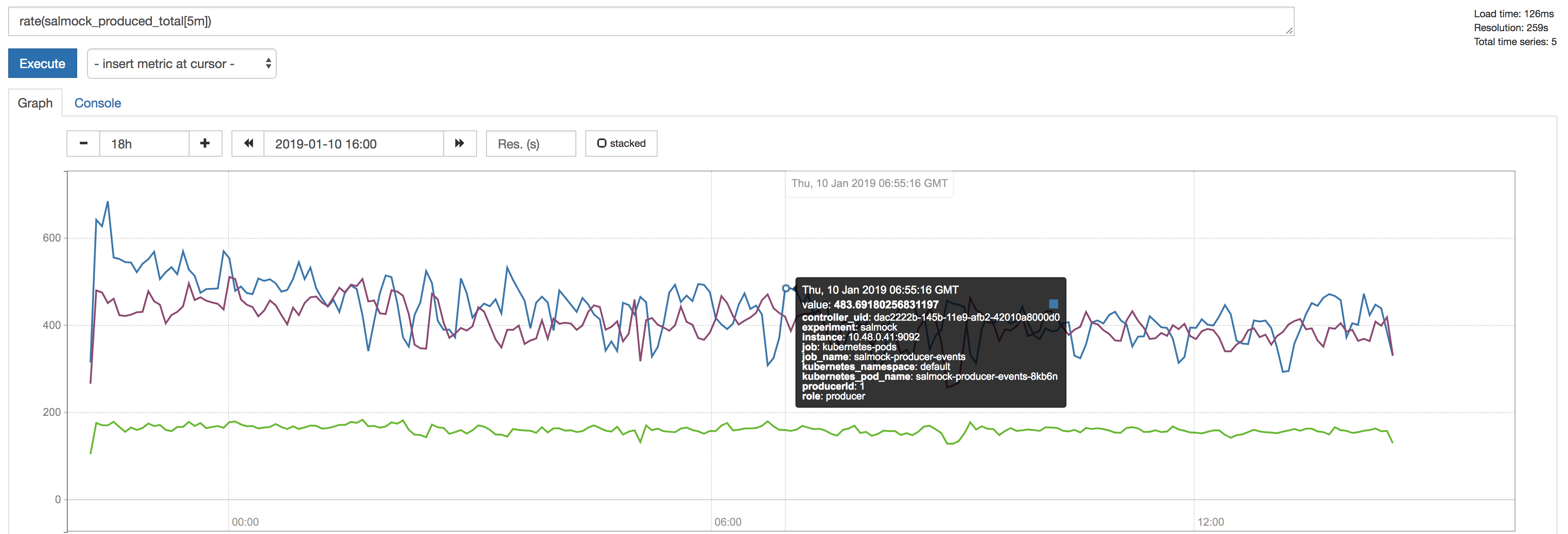
Figure 1 The figure shows the producer throughput measured by the salmock_produced_total Prometheus metric.
- Number of topics produced: 1051
- Maximum measured throughput for the producers: 1330 messages/s
Another Prometheus metric of interest is cp_kafka_server_brokertopicmetrics_bytesinpersec. This metric gives us a mean throughput at the brokers, for all topics, of 40KB/s. We observe the same value when looking at the Network traffic as monitored by the InfluxDB telegraf client.
As a point of comparison,the Long-term mean ingest rate to the Engineering and Facilities Database of non-science images required to be supported for the EFD of 1.9 MB/s from OCS-REQ-0048.
We can do better by improving the producer throughput, and we demonstrate that we can reach a higher throughput with a simple test when accessing the InfluxDB maximum ingestion rate for the current setup (see 6.4 The InfluxDB ingestion rate).
6.3 Latency measurements
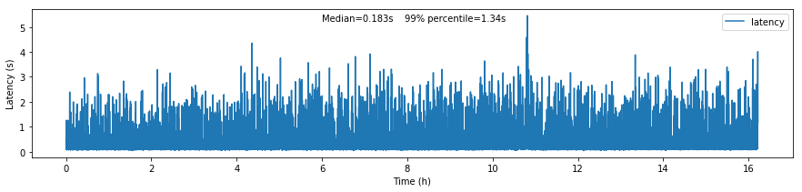
Figure 2 The figure shows the roundtrip latency for a telemetry topic during the experiment, measured as the difference between the producer and consumer timestamps.
We characterize the roundtrip latency as the difference between the time the message was produced and the time InfluxDB writes it to the disk.
The median roundtrip latency for a telemetry topic produced over the duration of the experiment was 183ms with 99% of the messages with latency smaller than 1.34s.
This result is encouraging for enabling quasi-realtime access to the telemetry stream from resources at the Base Facility or even at the LDF. That would not be possible with the current baseline design (see discussion in DMTN-082).
6.4 The InfluxDB ingestion rate
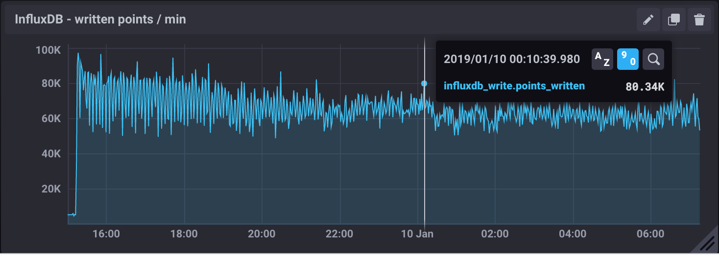
Figure 3 The figure shows the InfluxDB ingestion rate in units of points per minute.
The measured InfluxDB ingestion rate during the experiment was 1333 messages/s, which is essentially the producer throughput (see 6.2 Producing SAL topics). This result is supported by the very low latency observed.
Note
Because of the current InfluxDB schema, an InfluxDB point is equivalent to a SAL topic message.
InfluxDB provides a metric write_error that counts the number of errors when writing points, and it was write_error=0 during the whole experiment.
During the experiment, we also saw the InfluxDB disk filling up at a rate of 682MB/h or 16GB/day. Even with InfluxDB data compression that means 5.7TB/year which seems too much, especially if we want to query over longer periods like OCS-REQ-0047 suggests, e.g., “raft 13 temperatures for past two years”. For the DM-EFD, we are considering downsampling the time series and using a retention policy (see 8 Lessons Learned).
Finally, a simple test can be done to assess the maximum InfluxDB ingestion rate for the current setup.
We paused the InfluxDB Sink connector, and let the producer run for a period T. The Kafka brokers cached the messages produced during T, and as soon as the connector was re-started, all the messages were flushed to InfluxDB as if they were produced in a much higher throughput.
The figure below shows the result of this test, where we see a measured ingestion rate of 1M messages per minute (or 16k messages per second), a factor of 12 better than the previous result. Also, we had write_error=0 during this test.
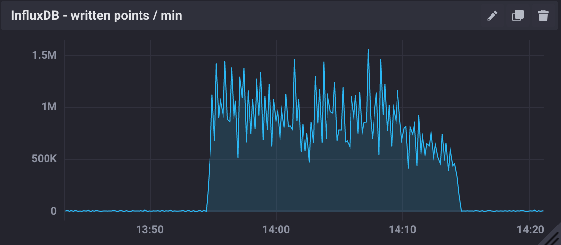
Figure 4 The figure shows the InfluxDB maximum ingestion rate measured in units of points per minute.
In particular, these results are very encouraging because both Kafka and InfluxDB were deployed in modest hardware, and with default configurations. There is indeed room for improvement, and many aspects to explore in both Kafka and InfluxDB deployments.
6.5 Visualizing SAL Topics with Chronograf
The Chronograf UI presents the SAL topics as InfluxDB measurements. One can use the Explore tool to browse and visualize them using the Query Builder to build a query that defines the visualization.
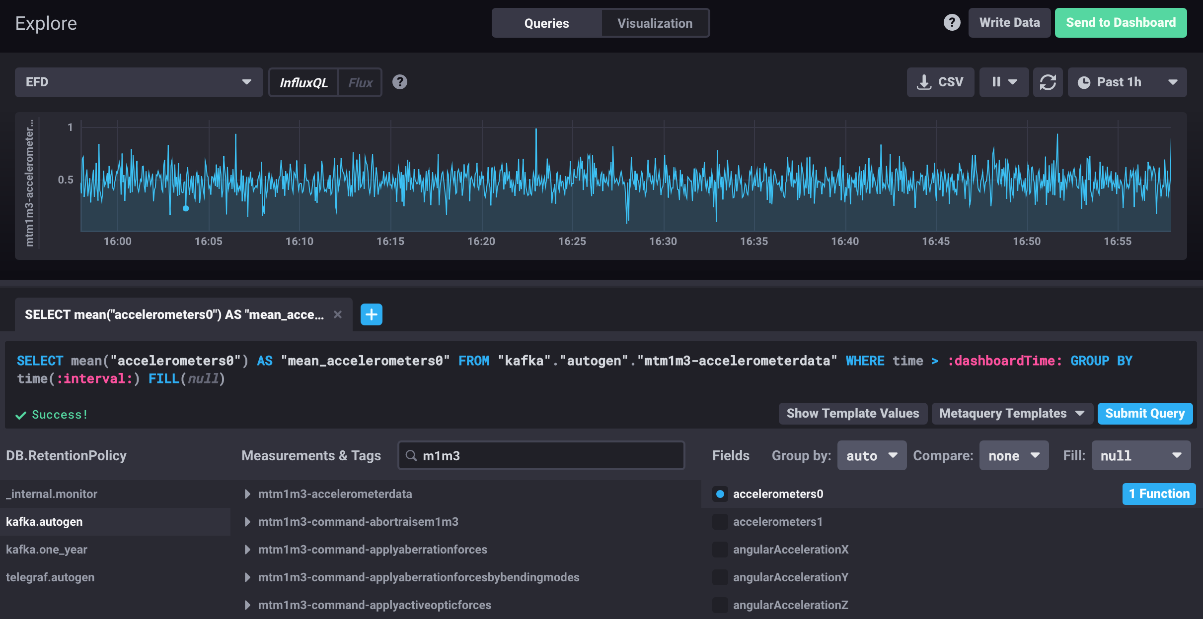
Figure 5 Visualization using the Chronograf Explore tool.
For monitoring the different telescope and observatory subsystems, it is possible to organize these visualizations in Dashboards in Chronograf.
The InfluxData stack was also adopted for the SQuaSH system, and it will be possible to access both DM-EFD and SQuaSH databases from the same Chronograf instance combining both telemetry and Science Quality data (see also 8.2 The InfluxDB HTTP API).
7 Live SAL experiment with Avro transformations
This experiment is a live demonstration of the full end-to-end DM-EFD using the mirror cell (MTM1M3 and MTM1M3TS subsystems) SAL simulator. SAL has implemented Kafka writers that produce plain text messages to Kafka topics named MTM1M3_telemetry and MTM1M3TS_telemetry.
The figure shows the set up for the experiment where the SAL M1M3 simulator runs in Tucson and the DM-EFD cluster at Google Kubernetes Engine (GKE).

Figure 6 Set up for the live SAL experiment with Avro transformations. The SAL M1M3 simulator runs in Tucson and the DM-EFD cluster at Google Kubernetes Engine (GKE).
Topics are simulated at 50Hz by the SAL simulator. They reach the Kafka brokers at the DM-EFD cluster.
Transformer applications, implemented as part of the kafka-efd-demo codebase and deployed to GKE consume these topics, parse the plain text messages, serialize the content with Avro, and produce messages to a second set of Kafka topics named after the fully-qualified names of the schemas within the lsst.sal. namespace. These topics are consumed by Kafka connect which uses the InfluxDB Sink connector to write the messages to InfluxDB.
The goal of this experiment is to verify if the online message transformation approach discussed in 4.5 Practical approaches to integrating Avro into the SAL and DM-EFD system can keep up with 50Hz telemetry stream.
7.1 Latency characterization
The latency for a specific topic was measured in different points of the system using the timestamps indicated in the figure. The end-to-end latency is given by sal_created - influxdb_timestamp.
Initial results showed that we were writing data to InfluxDB at ~20Hz when expected 50Hz.
We have improved the hardware configuration in our deployment compared to cluster-specs.
- Machine type: n1-standard-4 (4 vCPUs, 15 GB memory)
- Size: 4 nodes
- Total cores: 16 vCPUs
- Total memory: 60 GB
- Using SSD disks for Kafka and InfluxDB
Using SSDs disks and adding one extra node to have more resources for InfluxDB helped to improve the latency, but it became clear that the transformation step was the main bottleneck.
The latency measured by influxdb_timestamp - kafka_timestamp, does not including the transformation step, is compatible with the results presented before in 6.3 Latency measurements.
In particular, the time to consume, transform, and produce the message with the biggest payload in the experiment lsst.sal.MTM1M3_forceActuatorData essentially dictates the latency we observe.
7.1.1 Tuning the consumer and producer settings
We also found that the time to consume and produce the messages is comparable to the time to transform them. First we tuned the consumer and producer settings using check_crcs=False and ack=0 respectively. That reduced the time to consume-transform-produce `lsst.sal.MTM1M3_forceActuatorData messages from 0.05s to 0.035s
The transformation step includes the time to retrieve the schema from the Kafka Schema Registry, the time to process the message fields and the time to serialize to Avro, which are roughly 9%, 90% and 1% of the transformation time respectively.
7.1.2 Transform optimization
To reduce the time to process the message fields we introduced the --tasks option to SAL transform that creates a configurable asyncio buffer to process messages concurrently.
We found that --tasks 10 is enough to reduce the transform time by 10ms.
After running SAL transform with that option and disabling the debug logs we were able to keep up with the 50Hz telemetry stream.
The figure shows the end-to-end latency for lsst.sal.MTM1M3_forceActuatorData messages after running the experiment for 1h. After tuning the consumer and producer settings and optimizing the transformation step we measured a medium latency of 0.058s with 99% of the time below 0.36s.
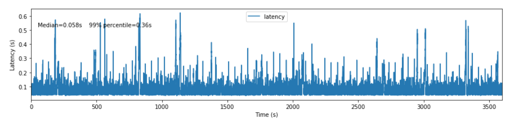
Figure 7 Latency measured after tuning the consumer and producer settings and optimizing the transformation step.
We also notice that querying the InfluxDB at the same time reduces the ingestion rate and introduces some latency, but after some time we are able to recover.

Figure 8 Latency measured after loading the InfluxDB with queries.
8 Lessons Learned
8.1 Downsampling and data retention
It was evident during the experiment that the disks fill up pretty quickly. The influxDB disk was filling up at a rate of ~700M/h which means that the 128G storage would be filled up in ~7 days. Similarly, for Kafka, we filled up the 5G disk of each broker in a few days. That means we need downsampling the data if we don’t want to lose it and configure retention policies to automatically discard high frequency data if it is no longer useful.
In InfluxDB it is easy to configure both downsampling and data retention.
InfluxDB organizes time series data in shards and will drop an entire shard when it enforces the retention policy. That means the retention policy’s duration must be longer than the shard duration.
For the experiments, we have created a Kafka database in InfluxDB to have a default retention policy of 24h and shard duration of 1h following the retention policy documentation.
InfluxDB creates retention policies per database, and it is possible to have multiple retention policies for the same database. To preserve data for a more extended period, we have created another retention policy with a duration of 1 year and demonstrate that a Continuous Query can be configured to average the time series every 30s. That lead to a downsampling factor of 3000 for topics produced at 100Hz.

Figure 9 The figure shows a raw time series (top) and an averaged time series by a continuous query (bottom).
Example of a continuous query for the mtm1m3-accelerometerdata topic.
CREATE continuous query "mtm1m3-accelerometerdata" ON kafka
BEGINSELECT   Mean(accelerometers0) as mean_accelerometers0,
           Mean(accelerometers1) as mean_accelerometers1
  INTO     "kafka.one_year"."mtm1m3-accelerometerdata"
  FROM     "kafka.autogen"."mtm1m3-accelerometerdata"
  GROUP BY time(30s)
END
The retention policy of 24h in InfluxDB suggests that we configure a Kafka retention policy for the logs and topic offsets with the same duration. It means that the database can be unavailable for 24h and it is still possible to recover the messages from the Kafka brokers. We added the following configuration parameters to the cp-kafka helm chart:
## Kafka Server properties
## ref: https://kafka.apache.org/documentation/#configuration
configurationOverrides:
  offsets.retention.minutes: 1440
  log.retention.hours: 24
8.2 The InfluxDB HTTP API
InfluxDB provides an HTTP API for accessing the data, when using the HTTP API we
set max_row_limit=0 in the InfluxDB configuration to avoid data truncation.
A code snippet to retrieve data from a particular topic would look like:
import requests

INFLUXDB_API_URL = "https://kafka-influxdb-demo.lsst.codes"
INFLUXDB_DATABASE = "kafka"

def get_topic_data(topic):
  params={'q': 'SELECT * FROM "{}\"."autogen"."{}" where time > now()-24h'.format(INFLUXDB_DATABASE, topic)}
  r = requests.post(url=INFLUXDB_API_URL + "/query", params=params)

  return r.json()
Following the desin in DMTN-082 we plan to access this data from the LSST Science Platform through a common TAP API, that seems possible using for example Influxalchemy.
8.3 Backing up an InfluxDB database
InfluxDB supports backup and restores functions on online databases. A backup of a 24h worth of data database took less than 10 minutes in our current setup while running the SAL Mock Experiment and ingesting data at 80k points/min.
Backup files are split by shards, in Downsampling and data retention we configured our retention policy to 24h and shard duration to 1h, so the resulting backup has 24 files.
We do observe a drop in the ingestion rate to 50k points/min during the backup, but no write errors and Kafka design ensures nothing gets lost even if the InfluxDB ingestion rate slows down.
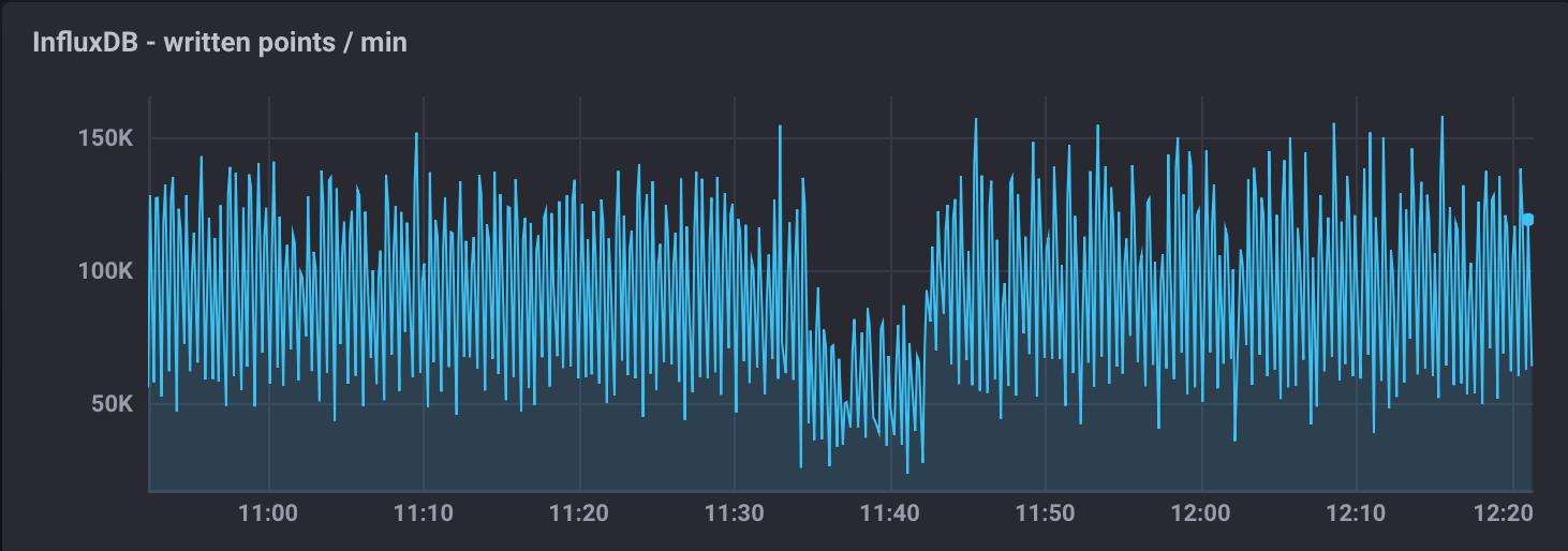
Figure 10 The figure shows how the InfluxDB ingestion rate is affected during a backup.
8.4 InfluxDB memory usage
Concerns about InfluxDB memory usage were raised in this community post. The original post use case is low load (~1000 series) in a constrained hardware 1 GB memory using InfluxDB 1.6.
We didn’t observe issues with memory usage in InfluxDB 1.7 during the SAL mock experiment. Memory usage was about 4GB for moderate load (< 1 million series) on a n1-standard-2 (2 vCPUs, 7.5 GB memory) GKE instance. That is compatible with the hardware sizing recommendations for single node (see InfluxDB hardware guidelines ).
However, we didn’t store the raw data for more than 24h in this experiment and did not try queries over longer time periods. For querying over long time periods, downsampling the data seems to be the only feasible option.

Figure 11 The figure shows memory usage and other statistics obtained from the Telegraf plugin deployed to the InfluxDB instance, during one of the experiments. The four curves displayed in the CPU usage are usage_system, usage_user, usage_iowait and usage_idle.
9 APPENDIX
9.1 DM-EFD play book
In this section we list commands and procedures that were useful during the implementation and tests of the DM-EFD.
9.1.1 Running the kafkaefd utility locally
Install kafkaefd on a virtual environment with Python 3.6+:
virtualenv env --python python3.6
source env/bin/activate
pip install git+https://github.com/lsst-sqre/kafka-efd-demo
You can run kafkaefd locally while connecting to the remote Kafka cluster on Kubernetes using Telepresence:
telepresence --run-shell --namespace kafka --also-proxy confluent-cp-kafka-headless --also-proxy confluent-cp-schema-registry --also-proxy confluent-cp-kafka-connect
Set the following environment variables used by kafkaefd:
export BROKER=confluent-cp-kafka-headless:9092
export KAFKA_CONNECT=http://confluent-cp-kafka-connect:8083
export SCHEMAREGISTRY=http://confluent-cp-schema-registry:8081
9.1.2 Listing topics
kafkaefd admin topics list
A SAL topic is prefixed by the subsystem name, and have a suffix identifying its type (command, telemetry or event).
Topics starting with lsst.sal. are produced by the SAL transform app. The corresponding Avro schemas are organized by subjects with the same name.
9.1.3 Deleting topics
For testing, sometimes, it is useful to eliminate the initial offset for the topics, you can do that by deleting them:
kafkaefd admin topics delete $(kafkaefd admin topics list --inline --filter MTM1M3*)
9.1.4 Debugging the SAL transform app
Inspecting the SAL transform logs for a particular subsystem:
kubectl logs $(kubectl get pods --namespace kafka-efd-apps -l "app=saltransform,subsystem=MTM1M3" -o jsonpath="{.items[0].metadata.name}") --namespace kafka-efd-apps
For debugging the SAL transform app, you might want to run it locally. In doing so, you should first delete the actual deployment in the cluster and then run the app locally.
kafkaefd saltransform run --auto-offset-reset latest --subsystem MTM1M3 --log-level debug
9.1.5 Debugging the InfluxDB Sink connector
Inspecting the Kafka connect logs:
kubectl logs $(kubectl get pods --namespace kafka -l "app=cp-kafka-connect,release=confluent" -o jsonpath="{.items[0].metadata.name}") cp-kafka-connect-server --namespace kafka -f
Checking the status of the influxdb-sink connector:
kafkaefd admin connectors status influxdb-sink
Deleting the influxdb-sink connector:
kafkaefd admin connectors delete influxdb-sink
Creating a new connector that consumes all the lsst.sal.* topics:
kafkaefd admin connectors create influxdb-sink --influxdb https://influxdb-efd-kafka.lsst.codes --database efd --username <influxdb username> --password <influxdb password> --daemon $(kafkaefd admin topics list --inline --filter lsst.sal.*)
9.2 Kafka Terminology
- A Kafka cluster can have several brokers, other components are the Schema Registry, the Zookeeper and the Kafka Connect.
- Kafka stores messages in a category name called topic.
- A Kafka message is a key-value pair. The key, message, or both, can be serialized as Avro.
- A schema defines the structure of the Avro data format.
- The Schema Registry defines a subject or scope where a schema can evolve. The name of the subject depends on the configured subject name strategy, which by default is set to derive the subject name from the topic name.
- The processes that publish messages to Kafka are called producers. Also, they publish data on specific topics.
- Consumers are processes that subscribe to topics.
- The position of the consumer in the log is called offset. Kafka retains that on a per-consumer basis.
- The Kafka connector permits to build and run reusable consumers or producers that connects existing applications to Kafka topics.
9.3 InfluxDB Terminology
- A measurement is conceptually similar to an SQL table. The measurement name describes the data stored in the associated fields.
- A field corresponds to the actual data and are not indexed.
- A tag is used to annotate your data (metadata) and is automatically indexed.
- A point contains the field-set of a series for a given tag-set and timestamp. Points are equivalent to messages in Kafka.
- A measurement and a tag-set define a series. A series* contains points.
- The series cardinality depends mostly on how the tag-set is designed. A rule of thumb for InfluxDB is to have fewer series with more points than more series with fewer points to improve performance.
- A database store one or more series.
- A database can have one or more retention policies.